Geeky Reviews – Madras Cafe via Twitter


It seems like I have been going south since the blog started, first with the politicians and then Chennai Express. So continuing that journey, this time around I am looking at a Madras Cafe to find out what the TwitterVerse has been talking about it. Now the process is pretty much similar to that of last time around (see Twitter Movie Review – Chennai Express), however there are two improvements. To start with the sample of Tweets is larger, I am looking at about 3000 tweets (3099 precisely) and the time span of the tweets is from 23rd August morning till 24th early morning. There are couple of ways this helps, first we are likely to see a broader verdict and second, the amount of noise in the tweets will be somewhat low. It also helps that I collected the data pretty soon after movie release and since the movie does not have as much PR & marketing blitzkrieg as Chennai Express,  the tweets are much less noisy and more diverse.

Word Cloud

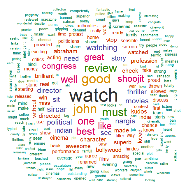
This is how #MadrasCafe verdict looks on a word cloud.

Madras Cafe, Review, Twitter, R, Text mining, tweetsent

TweetCloud Madras Cafe

Visually, it looks like Madras Cafe has got pretty good reviews and thumbs-up from a lot of folks who have seen it and tweeted about.  Words like “awesome”, “superb” ,”good”, “must watch”, are frequently associated with it. We also see a lot of appreciation and chatter about John Abraham who has produced the movie and acted as well. There is also a great deal of appreciation for the director Shoojit Sircar and Nargis Fakhri. We also see some words not directly related to the movie, which is perhaps the spillage from other topics that were being discussed or trending and were tagged #MadrasCafe.

Cluster Analysis

Cluster analysis is a nice way to get better insights into the data. It helps to understand which objects, in our case terms or words, are more associated with each other and which are far. So rather than just seeing  the most frequent terms, we can look at terms that frequently occur together in a tweet. This helps to get clear sense of what people are talking about when they use such terms. I have done some clean-up while ensuring that the structure of data remains intact. This is needed because first, there is a lot of noise in the data  and second, it is important to restrict cluster analysis to finding important chunks of objects that go together. More on this in the technical part.

Geeky reviews, Madras Cafe reviews, Twitter, Text mining, R, tm

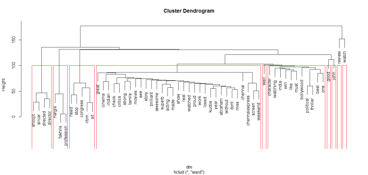
The above diagram is how the clusters looks like. I have divided the diagram in 10 clusters, indicated by red borders. The terms which occur higher in the clusters are the ones that occur more frequently and the terms which are close to each other are the ones which occur together.

We can get a lot more insight about the terms we saw in the Word Cloud when we look at the clusters in which they occur. So for example, the third cluster from the left is regarding the spillage I talked about earlier. Here we see the terms that occurred together and it looks like some trolls trying to get more visibility by using the Madras Cafe hashtag while tweeting about things not much related. The first cluster on the left is about the director, and the one next to it is some sort of discussion about Nargis Fakhri. However, such terms are slightly low on the diagram indicating that they are occurring relatively less frequently.

The terms “watch” & “review” on the top right are the ones that occur a lot more frequently and also occur together often. The reason for the two terms occurring more frequently is since the data was extracted during initial one or two days of the release, as a result there were a lot people who had watched or where planning to watch the movie. More importantly, this is also the time around which leading critics, newspapers and websites post their reviews and tweet about it and since they tend to have a lot of followers, such tweets get retweeted a lot and as a result the frequency of terms is higher.

The big cluster right in the middle is the one that we are most interested in. From the frequently occurring terms and the closeness of the terms, we can easily make out that this cluster is largely about the movie. Here we can confirm what we saw in the word cloud, the word “awesome”, “superb”, “kudos”, “brilliant” are frequently occurring with the words “story”, “acting”. Also there is some talk about Chennai Express, probably a comparison or something. There is also a second cluster towards the right which does seem to be related to the movie however it looks more generic perhaps talking about bollywood and Indian cinema in the context of this movie. Only two terms in this cluster seem directly related to the movie, “political” & “thriller”.

Sentiment Analysis

Now let us look at the overall sentiment expressed on Twitter for the movie, remember in the last review, we saw Chennai Express getting about 61% positive sentiment on Twitter. In comparison, below is the sentiment for Madras Cafe:

Positive Percentage: 72%

Comparing this largely positive sentiment with the reviews and ratings from other places:

TOI – 4/5

Rediff.com – 3.5/5

IMDB – 8.4/10

CNN-IBN – 3.5/5

Bollywood Hungama – 4/5

Again there is a close match between the sentiment from Twitter (specifically my code) and what is seen around the web. This is also in line with the word cloud and associations seen earlier.So in case you are geekily reading this review you might want to check out the movie as well. 🙂

I have talked more in-depth about the sentiment analysis method I adopted in my earlier post, so if you are interested do check it out here.

Long Tail

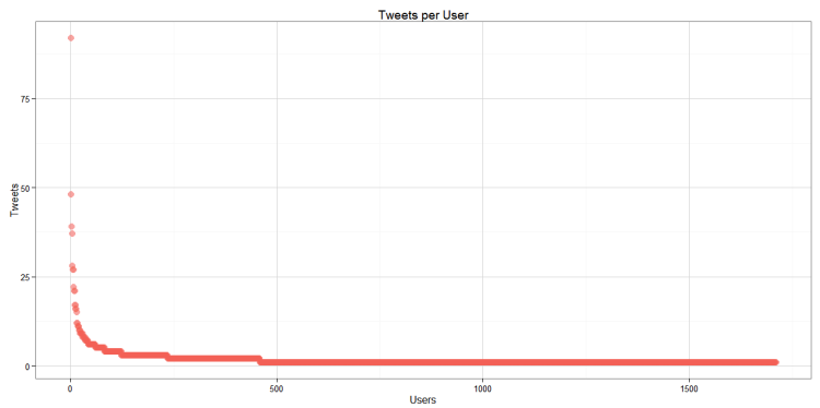
One last thing that I was interested in is the number of tweets per user. This will help to understand whether there are few individuals tweeting a lot or we have more diverse group. It is important since, there is a possibility that most of our tweets might come from a few users who happened to be tweeting a lot about this topic during the time we downloaded the tweets. In that case our data set will be biased and the analysis might not represent the true picture. So what we are hoping to see via this analysis is the long tail graph showing  many users tweeting in small amounts and only a few users with high number of tweets. Here is what we find in our case:

Long Tail, Madras Cafe Review, R, Tweetsent, Twitter

Here we clearly see a long tail that sharply tapers off and we have less than 10 users with more than 20 tweets about the topic. This is a good thing, as it indicates that the data we have does represent the opinion of many people and is not just a limited to few individuals

Without disclosing the screen names, the highest tweeter has about 92 tweets. Having checked out the tweets, it looks as if the user is trying to get people to read his review by tweeting a lot and tagging many people. Among the others, there are a lot of tweets for a contest by Inox and from Box Office Updates.

Finally, thanks for reading, if you like what you just read, please share and do leave your comment/suggestions/question/PJ/or code 😛 . Thanks….!

Technical Details:

The code is largely similar to last time and can be found at the end here.  However, there are couple of new additions, basically about the cluster analysis and the long tail.

In the cluster analysis, part I have used Hierarchical Agglomerative Clustering which is a part of core R package. I did do some pre-processing of the data before I did clustering. For this part I took the raw dataset and the not the one used for word cloud & sentiment analysis. The reason is that, while creating the word cloud, I just had words and their frequencies, everything else about the structure was largely lost. So I took the original data set, created a corpus which is basically a vector of tweets. After that I did some  clean-up of the data set, and converted the entire data set into the term-document matrix. A term-document matrix is basically a matrix which describe the frequency of terms occurring in each of the documents, here the documents are tweets. The advantage of term document matrix is that it preserves the structure of the tweets.  After this another thing that I did was, I removed all the sparse term to reduce the sparsity percentage, since twitter data contains a lot of noise, this is an essential step or else our clusters will not come out properly. Finally after this and lots of errors, I created the cluster. Here is the code for that part:

</p>
#Association and cluster analysis

mc.corpus <- lapply(mcafe, function(x) x$getText())

#removes retweets,RT@ etc.
mc.corpus <- lapply(mc.corpus, function(x) gsub("[@][^ ]*", " ", x))

#removes url's
mc.corpus <- lapply(mc.corpus, function(x) gsub("[h][t][t][[p][^ ]*", " ", x))
# Creating corpus

mc.corpus <- Corpus(VectorSource(mc.corpus))

mc.corpus <- tm_map(mc.corpus, tolower)

mc.corpus <- tm_map(mc.corpus, removePunctuation)

mc.corpus <- tm_map(mc.corpus, removeWords, stp)

mc.corpus <- tm_map(mc.corpus, removeNumbers)

mc.dtm <- TermDocumentMatrix(mc.corpus)

mc.dm <- removeSparseTerms(mc.dtm, sparse= 0.985)

mc.df <- as.data.frame(inspect(mc.dm))

#Creating Hierarchical Clusters
mc.scale <- scale(mc.df)

dm <- dist(mc.scale, method = "euclidean")
clust.mc <- hclust(dm, method = "ward")

plot(clust.mc)

groups <- cutree(clust.mc, k = 10)

rect.hclust(clust.mc, k = 10, border = "red")

The process of creating the long tail was pretty simple, I simply extracted the Screen Names, created a table and sorted them frequency. Post this I plotted the screen names to get the graph that we saw. Here is the code for that:


# Long Tail of Users

usr <- read.csv(file = "X:/TweetSent/mcafe.csv")

users <- as.data.frame(table(usr$screenName))

colnames(users) <- c("user", "tweets")

user.sort <- users[order(-users$tweets),]

library(ggplot2)

p <- qplot(1:nrow(user.sort), tweets, data = user.sort, color = "red", alpha = 0.25, size = 4, geom = "point", main = "Tweets per User", xlab = "Users", ylab = "Tweets")

p + theme_bw()
Twitter Movie Review – Chennai Express


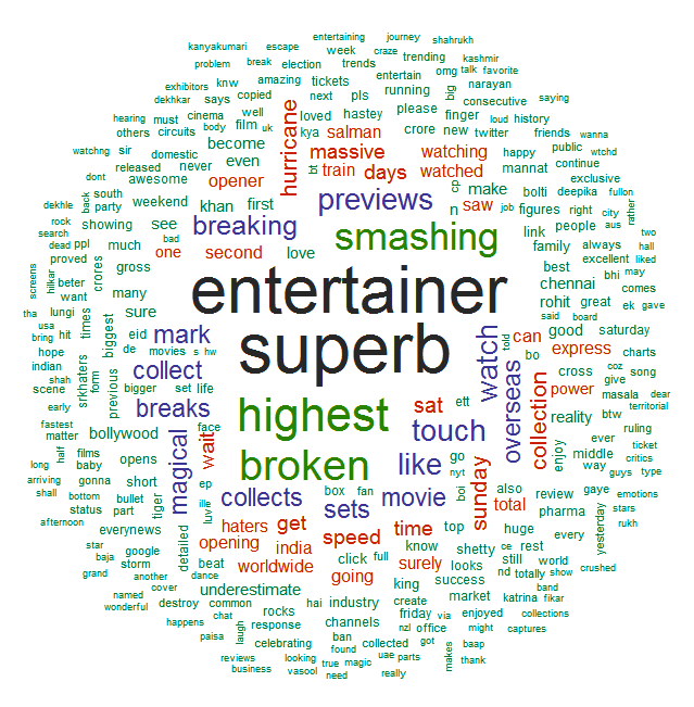
In the spirit of my first post (Pappu Vs. Feku) I will continue to explore the use of Twitter in providing an eye into the events of contemporary interest, and movies are certainly something that capture interest of a large majority of Indian audience. So I am looking at Chennai Express that released last week and has been generating all kinds of buzz both online and offline. The idea is to come up with some sort of review of the movie by fetching the tweets about the movie and analyzing them by using a R code. So I managed to pull about 1500 (Note: This is the maximum Twitter API limit) tweets that were directly talking about the movie. After doing a bit of clean-up and removing terms not helpful for review purposes (read: Karan Johar and Taran Adarsh), this is how the whole Twitter chatter about Chennai Express looks like:

twitter-movie-review-chennai-express

Chenna Express on Twitter

For those who are interested in seeing a table, here is the list of top ten five frequent terms:

Word Frequency
Superb 195
Entertainer 188
Highest 120
Broken 109
Smashing 98

Now since this review comes almost three days into the movie, in the tag cloud we see a lot of talk about the collection of the movie, however we can easily see the movie has been described by a lot of people as superb and entertaining. This is in line with the huge box office success that the movie has turned out to be.

Obviously such an approach only shows the loudest voices and can easily masquerade the overall opinion. Thus to be somewhat more nuanced, I have drilled down a bit further and did some sort of sentiment analysis. To keep things simple I have just examined the sentiments in terms of positive and negative. I basically break down all the tweets into individual words and create a sentiment score by classifying them as positive or negative. For classification purposes I am using Hu and Liu’s lexicon of 6800 words found here. Without getting too much in two technical details, below is the sentiment score I could calculate.

Positive Percentage : 61%

It must be noted that this number based only on positive and negative words in the tweets and ignores large number words which do not really express either positive or negative sentiment. Also I have no way of accounting of sarcasm or vernacular words and phrases. But I think that overall, the number of such instances is likely to be less than 15%. However going ahead I would also want to include a map of clusters of words that go occur together more often in order to get a better idea.

So with this score let us compare with what other popular reviews say about Chennai Express:

IMDB – 7.5/10

Rediff.com – 3/5

Yahoo – 3/5

Bookmyshow – 3.5/5

It looks like my Twitter review has done decently well as compared to the above, however the real test would be to do this analysis on the day of the release or the next morning and make some prediction about success of the movie. Going forward, this is going to be the idea and I will provide an analysis of one or two movies per week  and maybe I will be able to come up with some decent predictor of movie performance beforehand. Obviously such a review can never go into the nuances of the film and frankly it is not even intended here, the idea is just to explore how much can be understood from the opinion on Twitter and see how it tallies with the reality. Let me know your thoughts and ideas in the comments section.

Technical Details:

If you have read my first post (I suggest you do, at least the technical part) than basically this is just an extension of that. About fifty percent of the code is still the same, I have tried to be more nuanced when it came to stop words, to do that I just created a quick and dirty tag cloud and based on that expanded the list of stop words. Also unlike last time, I have removed all the screen names/ user names, since popular names tend to create a lot more noise and add little value. Finally, the sentiment analysis code is heavily influenced from couple of sources online which I mention in the end.

Code:


library("ROAuth")
 library("twitteR")
 library("RJSONIO")
 library("wordcloud")
 library("tm")
 library("plyr")
 library("stringr")

load("twitter authentication.Rdata")

registerTwitterOAuth(twitCred)

#searchTwitter for Movie -Chennai Express here

movie <- searchTwitter('#ChennaiExpress', n = 1500,lang = 'en', cainfo = "cacert.pem")

save(movie, file = "X:/TweetSent/ce.Rdata")

ce <- twListToDF(movie)

write.csv(ce, file = "X:/TweetSent/ce.csv")

#test to remove numbers as well

test <- strsplit(ce$text, " ")

stp <- stopwords("en")

#Customizing stop words list

stp <- c(stp, 'record','till', 'hey', 'thu', 'paid', 'now', 'fri', 'nett', 'breakdown', 'meant', 'last', 'ke', 'ki', 'par', 'r', 'ur', 'aur', 'pic', 'sun', 'beautiful','last','celebration', 'justified', 'done', 'd', 'dat', 'u', 'say', 'rs', 'records', 'cr', 'gauri', 'thats', 'will', 'needs', 'just', 'fans', 'day', 'srk', 'today', 'crs')

movie_test <- lapply(test, function(x) x[grep("^[[:alpha:]]+$", x)])

movie_test <- unlist(movie_test)

movie_test <- tolower(movie_test)

movie_test <- movie_test[-grep("^[rm]t$", movie_test)]

movie_test <- movie_test[!movie_test %in% stp]

movie.ts <- as.data.frame(table(movie_test))

movie.ts <- movie.ts[sort.list(movie.ts$Freq, decreasing = T),]
 print(xtable(head(movie.ts, 10),caption = "Top 10 words in tweets"), file = "X:/TweetSent/tabletest", include.rownames = F)

#Selecting color palettes for wordcloud

library(RColorBrewer)
 pal2 <- brewer.pal(8,"Dark2")

wordcloud(movie.ts$movie_test, movie.ts$Freq, scale = c(4, 0.5), min.freq = 5, random.order = F, colors = pal2)

#Sentiment analysis on movie.ts

#Downloaded list of positive & negative words (about 6800) from http://www.cs.uic.edu/~liub/FBS/sentiment-analysis.html

pos <- scan("X:/TweetSent/opinion-lexicon-English/positive-words.txt", what = 'character', comment.char = ';')

neg <- scan("X:/TweetSent/opinion-lexicon-English/negative-words.txt", what = 'character', comment.char = ';')

#Sentiment Scoring Algorithm

words <- movie_test

score.sentiment = function(words, pos, neg, .progress='none')
 {

require(plyr)
 require(stringr)

#final <- matrix('', 0 ,3)

words <- movie_test

scores = laply(words, function(words, pos, neg) {

# comparing words with the downloaded lexicon

positive <- match(words, pos)
 negative <- match(words, neg)

positive <- sum(!is.na(positive))
 negative <- sum(!is.na(negative))

score <- c(positive, negative)
 #newrow <- c(words, score)
 #final <- rbind(final, newrow)

return(score)

}, pos, neg, .progress=.progress )

scores.df = data.frame(score = scores, text = words)

return(scores.df)
 }

final <- score.sentiment(words, pos, neg)

colnames(final) <- c("Positive", "Negative", "Word")

pos.percent <- sum(final$Positive) / (sum(final$Positive) + sum(final$Negative))

print(pos.percent)

Acknowledgements:

Twitter Coverage ISMB

First Shot: Sentiment Analysis in R

R Tutorial on Twitter text Mining

Pappu Vs. Feku – Twitter Wars


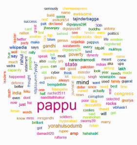
In my quest to practice R and learn text mining, I am looking at one of the popular Twitter Wars between two political personalities of India who are fondly known in the TwitterVerse as ‘Pappu’ and ‘Feku’ which is basically their ‘ghar ka naam’ or ‘pyar wala naam’. Anyway, the discussion about the origin of the names is beyond the scope of this post. What I was interested in finding out is what do people talk about or rather tweet about when they are fondly remembering these two prominent personalities. In order to do this I wrote a text mining program in a popular & open source language called R (technical details & code shared later in the post). For this purpose I used #pappu & #feku to fetch the relevant tweets. I was able to fetch about 1089 tweets for #pappu and about 1140 tweets for #feku.  After removing the common words (stopwords) like ‘and’, ‘is’ ‘are’, ‘the’, etc. I created a wordcloud to visually represent the data. To reduce noise and get a better less cluttered picture, only those words which featured at least 10 times (min. freq = 10) were selected. Below is what I found.

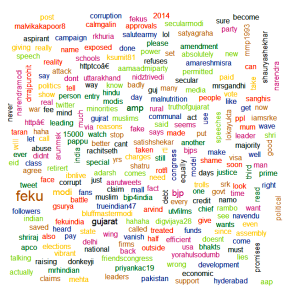
pappu2    feku2

The words which are in bigger font sizes are the ones that occur the most.  Also the words of same size and colors are the ones that have same frequency. For example in the case of #pappu, state & mind are the most frequently occurring terms. It is also important to note that the Twitter data is basically temporal and the value of insights derived tends to decay quickly overtime.

Anyways, here we see the most popular words, associated with #pappu & #feku. First thing that comes to mind is the fact that, there is more diversity in tweets about #feku. The most likely reason is that the said personality has been active in the political life a lot longer, has done & said many more things, thus giving more things to tweet about and more room to criticize or lament on the other hand, there is not much to criticize about #pappu because there nothing really been done apart from  statements & comments here and there.

There are many other obvious things here and one can really see how the two camps are trying to politically define the two. In case of #pappu it his recent comments as well as the controversy about in-laws and family in general. For #feku it is largely about the his claims of development, and allegations about his communal image. In both cases, the discourse is shaped and driven by the political opinions in the mainstream narrative about the two personalities.

One really interesting thing (interesting because I did not anticipate it :P) that came out here was the fact that I was also able to get information about the most enthusiastic/active tweeters of the both #pappu and #feku. So you notice various twitter handles also in the word cloud, well basically these are the handles which tweet a lot with the given hashtags. One can simply search these handle on Twitter to find out more, give it a try some might surprise you.  It  also might be worth exploring how much of the overall tweet content is driven by such users and how much is unique, however this would be the subject of the post.

Overall I wish to track this over the course of time and see how the discourse is shaped as we near general elections in 2014, keep watching. Let me know your thoughts, comments and ideas.

Technical Details:

To construct the above, I used three important R packages – TwitteR, tm and wordcloud along with RJSONIO and RcolorBrewer.

Unfortunately I was not able to fetch 1500 tweets, this might have to do something with the restrictions on get API in Twitter

Below is the code:


<em>library("ROAuth") #OAuth for twitter API</em>
 <em>library("twitteR")</em>
 <em>library("RJSONIO") #To resolve issues with JSON format, only load this after loading TwitteR</em>
 <em>library("wordcloud")</em>
 <em>library("tm")</em>

<em>#directly loading saved authentication file</em>
<em>#load("twitter_auth.Rdata")</em>

<em>#necessary step for Windows</em>
<em>download.file(url="http://curl.haxx.se/ca/cacert.pem", destfile="cacert.pem")</em>

<em>#Registering on Twitter API, only first time</em>

<em>reqURL <- "https://api.twitter.com/oauth/request_token"</em>
<em>accessURL <- "http://api.twitter.com/oauth/access_token"</em>
<em>authURL <- "http://api.twitter.com/oauth/authorize"</em>

#To fetch your consumer key go to https://twitter.com/apps/new and log-in ,read TwitteR documentation for details

<em>consumerKey <- "dummy"</em>
<em>consumerSecret <- "dummy"</em>
<em>Cred <- OAuthFactory$new(consumerKey = consumerKey, </em>
<em> consumerSecret = consumerSecret, requestURL = reqURL,</em>
<em> accessURL = accessURL, authURL = authURL)</em>

<em>Cred$handshake(cainfo = "cacert.pem")</em>

<em>#IMPORTANT: Run till the above line first, PIN will be asked, enter PIN & proceed</em>
<em>#save for later uses & fetch using load as mentioned above</em>

<em>save(Cred, file = "twitter_auth.Rdata")</em>

<em>registerTwitterOAuth(Cred)</em>

<em>#searchTwitter for Pappu</em>

<em>pappu <- searchTwitter('#pappu', n = 1500,lang = 'en', cainfo = "cacert.pem")</em>

<em>pappu <- sapply(pappu, function(x) x$getText())</em>

<em>pappu_corpus <- Corpus(VectorSource(pappu))</em>

<em>pappu_corpus <- tm_map(pappu_corpus, tolower)</em>

<em>pappu_corpus <- tm_map(pappu_corpus, removePunctuation)</em>

<em>pappu_corpus <- tm_map(pappu_corpus, function(x) removeWords(x, stopwords()))</em>

<em>#Selecting color palettes for wordcloud</em>

<em>library(RColorBrewer)</em>

<em>pal2 <- brewer.pal(8,"Pastel2")</em>

<em>wordcloud(pappu_corpus, scale = c(4,1), min.freq = 10, random.order = T, random.color = T, colors = pal2)</em>

<em>#searchTwitter for feku</em>

<em>feku <- searchTwitter('#feku', n = 1500,lang = 'en', retryOnRateLimit = 120, retryCount = 5, cainfo = "cacert.pem")</em>

<em>feku <- sapply(feku, function(x) x$getText())</em>

<em>feku_corpus <- Corpus(VectorSource(feku))</em>

<em>feku_corpus <- tm_map(feku_corpus, tolower)</em>

<em>feku_corpus <- tm_map(feku_corpus, removePunctuation)</em>

<em>feku_corpus <- tm_map(feku_corpus, function(x) removeWords(x, stopwords()))</em>

<em>wordcloud(feku_corpus, scale = c(2,1), min.freq = 10, random.order = T, random.color = T, colors = pal2)</em>

Acknowledgements:

I have learned the above largely from:

Text Data Mining With Twitter and R

Mining Twitter with R

Using the R TwitteR package

One R Tip a day

R Bloggers